Designing Data Intensive Applications - Partitioning

We previously discussed replicating our data, which has multiple benefits, one being allowing a higher read throughput. But to allow even higher read and write throughput, we need to partition our data, that is to split it into smaller parts and distribute these parts across multiple nodes.

Partitioning allow for greater scalability, as partitions can be distributed across multiple nodes, which also allows for higher availability.

Queries operating on a single partition can be executed more efficiently, as the data is smaller, and can be stored on a single node.

Larger and more complex queries can be executed by querying multiple partitions in parallel.

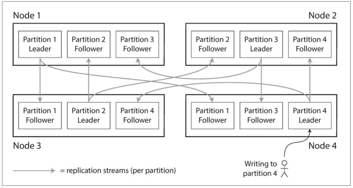
Partitioning and replication are usually used hand in hand. A node may store more than one partition, and each partition may be stored on multiple nodes.

In a leader-follower replication model, each partition’s leader will be follower for other partitions. It will look like the following:

Partitioning of key-value data #

There are some common pitfall with partitioning, one being data skew: If the partitioning of the data is unfair, that is, done on criteras that distribute the data across multiple partitions unevenly, some nodes will end up holding larger chuncks of the data than other ones.

Data skews will usually leads to another pitfall of partitioning: hot spots. A hot spot is when a partition suffer from a dispropotionate load in comparison to the other ones. The node holding the partition that is a hotspot will have higher ressources usage, which will cause unstability in the system and descrease the scalability.

One easy way to avoid hot spot would be to assign the records in the partitions randomly, but as there would be no way to know which partition to query to retrieve a given record, we would end up querying all the partition, so, too many nodes.

Partitioning by key range #

A simple way to partition data, is doing so by key range. That is, for a choosen key, assign certain ranges of it to partitions.

It is exactly the same as how encyclopedias often split themselves, in different volumes. For instance, the first volume covering topics from A to C, the volume 2 from D to F, etc…

It is not too hard to see where key range paritioning will be problematic: In a lot of cases, key ranges may leads to data skews & hot spots.

If we were to distribute the user profiles of a social media application over partitions, using the first name of the user as the key range, we will end up with some partition like the ones for X, Y or Z being way smaller than the ones for the letters A, M or T.

The boundaries may be chosen manually, or automatically by database systems.

Paritioning by key range can be extremely useful in some cases if we can predict that we will be querying only or very few partitions thanks to it. For instance, if we partition a data lake using the timestamp of the records as key, and create one partition for each day. To retrieve the data of a given day, we will predictably query only the necessary data.

Partitioning by hash of key #

As paritioning by key range is very much prone to data skew and hot spots, many distributed datastores use a hash function to determine the partition of a given key.

A good hash function for the partition keys will uniformly distribute skewed data.

A cryptographically strong hash function has the following properties:

• One-way function: It is computionally infeasable to find the input from the output
• Collision resistance: Extremely difficult to find to inputs that produces the same output
• Avalanche effect: Small changes in the input produces large changes & unpredictable in the output
• Uniformity: Output are evenly distributed
• Unpredictablity: Output cannot be predicted without computing the entire function

But, when hashing the partition key for a storage, we only need to comply with the following criteras :

• Uniform distribution
• Deterministic routing (The same key always return the same value/route to the same partition)
• Stability across processes/instances (The function must return the same value for a key regardless of which server process computes it, unlike Java’s hashCode() or Ruby’s hash)

So, going for a non cryptographycally strong function, like MD5 as used in Cassandra or MongoDB allows good distribution properties while avoiding a good overhead of cryptographically strong functions.

With that hash function, we can now associate each partition a range of hash. Now every key will be hashed, which will return a value corresponding to a partition.

One caveat with this method is that if we add or remove a partition, we will need to rehash all the keys, which can be expensive. This is called the partitioning problem. To solve this problem, we can use a technique called consistent hashing, which allows us to add or remove partitions without having to rehash all the keys (we’ll talk about it later).

Also, we unfortunately lose the ability to do range queries by using partition by hash of key. As we cannot know which partition to query for a given range of keys.

One compromise bewteen these solution, is to use a compound key, which is a combination of the partition key and a secondary key. This allows us to do range queries on the secondary key, while still using the partition key for partitioning. For instance, we could use for primary key (user_id, update_timestamp), choosing the user_id as the partiton key, and the timestamp as the secondary key. This would allow us to do range queries on the timestamp, while still partitioning the data by user ID. We will be able to query all the data for a given user, and then do range queries on the timestamp for that user.

Skewed workloads and relieving hot spots #

When partitioning data, we need to take into account the workload that will be done on the data. If we have a skewed workload, we may end up with hot spots independently of the partitioning method we use (if all the reads or writes concern a single user for instance).

One common solution is to identify such hot keys, and to split them over multiple partitions by adding a random suffix/prefix to the key. This way, we can distribute the load across multiple partitions, while still being able to query the data for a given user.

But this has the drawbacks of now requiring to read from multiple partitions to get the data for a given user. Aswell as requiring addititional bookkeeping of the keys judged as hot keys.

Partitioning and secondary indexes #

So far, it was pretty straightforward to determine the partition from a key and using it as a route for read and writes since it was the only access path to the data evoqued.

Things are more complicated when secondary indexes are involved. Secondary indexes are used to query data using a different key than the primary key. For instance, if we have a table of users, we may want to query the data using the email address of the user as a secondary index.

The secondary index don’t map neatly to the partitions, as the data is not stored in the same order as the secondary index. This means that we need to be able to query all the partitions to get the data for a given secondary index.

There exists two main ways to handle secondary indexes in a partitioned database.

Local indexes #

Local indexes, also known as document-partitioned indexes, are indexes that are stored on the same partition as the data. This means that the index is only valid for the data in that partition. One partition’s index have no idea of the data in another partition.

This issue is that, in most cases, unless something special was done on the document’s key, there is no reason that all the data for a given secondary index is stored in the same partition. So, when querying upon a secondary index, we need to query all the partitions, and then merge the results together. This is called a scatter-gather query. This can be quite expensive for large datasets.

Global indexes #

Global indexes cover all the partitions’s data. This means that the index is valid for all the data in the database. This allows us to query the data using the secondary index without having to query all the partitions.

However, as we are dealing with distributed systems, the global index also cannot be stored on a single node. It needs to be partitioned, but differently from the data. The partition strategy will depend on the access patterns of the data, but we can imagine for a simple case of a secondary index on the color of a car, we could partition the index by color, when the data is partitioned by the car’s ID.

This is also called as term-partitioned indexes, and it has the advantage of making the reads way more efficient, as we now can query only the partition that holds the relevant data for us.

The downside of it however, is that writes are now more expensive and complex, as we need to update the index in multiple partitions. This is called index maintenance overhead.

In theory, the index would reflect the data at all time, which means that the index needs to be updated every time a record is inserted, updated or deleted. This can be quite expensive for large datasets.

In practice, global secondary indexes are often maintained asynchronously, which makes it eventually consistent.

Rebalancing partitions #

Overtime, as:

• The data grows
• The throughput are increasing
• The access patterns change
• A machine fails

We will need to add or remove partitions, which forces the cluster to rebalance the data across the partitions. This is called partition rebalancing.

Basically, it is the process of redistributing the data across the partitions, so that each partition has roughly the same amount of data and load.

Not only we expect the data to be evenly distributed after a rebalancing, but this process shouldn’t cause any downtime both for the reads and writes. All that, while moving the least amount of data between nodes to make the rabalancing fast and minimize network & Disk I/O load.

Strategies for Rebalancing #

The wrong way: hash mod N #

Earlier, we discussed how it is best to divide the possible hash of values into ranges and assign the ranges to partitions.

This maybe rose the question of why we don’t just use the mod of the hashed key, modulo the number of partitions.

This unfortunately makes rebalancing way too expensive, as it would require to move most of the data between partition when adding or removing a node. For instance, if we have 4 partitions, and we add a 5th one, we would need to reassign and move 80% of the data.

Fixed numbers of partitions #

One simple solution to prevent the need of moving around too much data over a rebalancing, is having many more partitions than there are nodes. For instance, in a cluster of 10 nodes, we could have 1000 partitions, which would allow one new node in the cluster to be added, and it would simply “steal” entire partitions from the other nodes. In this example, only ~9.1% of the data would need to be moved around.

In this solution, the number of partition is usually fixed when the cluster is created, and it is not changed afterwards. Splitting partitions is technically possible, but operationally complex, and often not even implemented in the databases systems.

Each partition has an additional overhead, so having too many partitions can lead to performance issues. But, having too few partitions can lead to hot spots and data skews. So, it is important to find a good balance between the number of partitions and the number of nodes in the cluster.

Dynamic partitioning #

A fixed number of partitions would be inconvenient for databases using key range partitioning, as a wrong choice of partition boundaries can lead to data skews and hot spots.

Dynamic partitioning is a solution to this problem, where the number of partitions can be changed dynamically, as the data grows or shrinks.

One way to implement this, is splitting a partition when it reaches a certain size. e.g: if a partition reaches 10GB, it is split into two partitions, each holding half of the data.

We can also merge partitions when they are too small, e.g: if a partition is smaller than 1GB, it is merged with another partition.

Each partition is assigned to one node, and each node can handle multiple partitions. This allows us to add or remove nodes in the cluster without having to move too much data around.

Dynamic partitioning is more complex to implement than fixed partitioning, but it allows for more flexibility and better performance in the long run. It is not only suitable for key range partitioning, but also for hash partitioning. For instance, it is supported by MongoDB since the version 2.4, which support both key range and hash partitioning. In both cases the partitions are split and merged dynamically.

Partitioning proportionally to nodes #

Another option, is to have make the number of partitions proportional to the number of nodes in the cluster, that is, having a fixed number of partitions per node.

For instance, if we have 10 nodes, and we want to have 100 partitions, each node would hold 10 partitions. And if we add a new node, it will randomly choose 10 partitions to take from the other nodes, and take a split of the data in these partitions.

Operations: Automatic or Manual Rebalancing #

Automatic rebalancing are convenient as they don’t need much operational work. But it is still an expensive operation, in regards to the rerouting, and moving a large amount of data.

Combining automatic rebalancing with automatic failure can represent a risk, for example, if a node is slow to respond due to overload, it may be considered as failed, and a new node is added to the cluster. This would cause the automatic rebalancing to kick in, and the new node would take some partitions from the slow node, which would cause even more load on the system.

It can be a good thing to have a human in the loop to do rebalancing.

Request Routing #

The more general problem of discovery encompass the question that is “how can a client find the address of a service it wants to connect to?”. Especially in a distributed system, where services may move around between machines, or where the number of instances of a service may change dynamically, there are rabalancings, etc…

There exists few high-level solutions to this problem, such as:

• Allowing clients to contact any node (e.g via round-robing load balancing). If the requested node owns the partition the client is looking for, it will return the data. If not, it will redirect the client to the correct node.
• Using a central service registry, where each service registers itself with its address, and the clients can query the registry to find the address of the service they want to connect to. This is a partition-aware load balancer.
• Requiring the clients to know the partitioning and the routing logic, so they can compute the address of the node they want to connect to.

Apache Zookeeper is a popular service registry, which is used by many distributed systems, such as Apache Kafka (before 2.8.0) to manage the configuration and the discovery of services. It is a distributed key-value store that provides a simple API for clients to read and write data.

Cassandra uses a different approach: a gossip protocol which distributes the information about the nodes in the cluster to all the nodes. This way, any node can answer the client’s request, and redirect it to the correct node if necessary.

Summary #

Partitioning is crutioal to scale a distributed system, as it allows to distribute the data across multiple nodes, and to handle larger datasets and higher throughput.

It distributes the data across multiple nodes, which allows for greater scalability and availability. It also allows for higher read and write throughput, as queries can be executed in parallel on multiple partitions.

Choosing the right partitioning strategy is crucial, as it can lead to data skews and hot spots if not done correctly. The most common partitioning strategies being:

• Partitioning by key range
• Partitioning by hash of key
• Partitioning by compound key

Partitioning data that is accessed by secondary indexes is more complex, as it requires maintaining either:

• Local indexes, which are stored on the same partition as the data, but require querying all partitions to get the data for a given secondary index.
• Global indexes, which cover all the partitions’s data, but require maintaining the index in multiple partitions, which can be expensive.

Rebalancing and routing strategies are also important to ensure that the data is evenly distributed across the partitions throught time, and that the clients can find the correct node to connect to efficiently.